With all the retail software systems, integrated point of sale and inventory around, you’re likely tempted to indulge in complicated sales metrics.
Stop now! Or at least postpone it.
Consider focusing on just 5 essential retail sales metrics, before your mind is buried in Excel pivot tables or your Qlikview screen overcrowds and freezes. For all an all, it’s the real-time overview you need. Your way to glory is keeping real-life events running smoothly in real time, and adjusting your strategy after certain periods.
1. Number of Customers (Customer Traffic)
A number of customers are the most straightforward metric for your retail business. Even a child gets that the place that’s crowding with customers must be doing good. You normally don’t go to an empty restaurant, don’t you?
Customers are the sole source of money for your retail business. As Karl Marx had it, human work adds real value to land and capital. For a retailer, the more potential customers you get into your shop, the more money they’ll likely leave behind.
If you’re in e-commerce, measuring customer numbers is pretty easy. It does, however, take some experience in reading the analytics. Most probably you’ll be using Google Analytics, but don’t forget that your e-commerce backend has at least some visitor statistics. Even if these are not as fancy as Google provides, they are typically easy to read and might even be more accurate. Set your benchmarks, compare results to last year and yesterday.
In brick-and-mortar, pay attention to the number of visitors and the number of customers. The latter can be seen from your point of sale history. Use loyalty programs, so your customers identify themselves at the counter, then it’s much easier to understand if your retail traffic. Wait! Do you visit your retail stores in person? Visual estimation can be adequate enough. Estimate, before you start counting.
NB! A number of customers are the only metric you can grow almost infinitely, i.e. the theoretical limit is the number of inhabitants on Earth. And possibly more, depending on your views on extraterrestrial retail.
2. Effectivity (Retail Conversion Rate)
Alright, we already had to distinguish retail visitors and retail customers. Some visitor doesn’t buy anything. It’s rather unlikely in a big shopping mall, but very common in specialty stores or luxury boutiques.
In e-commerce, we’re talking about customer conversion ratio. This shows how many visitors a retailer turns into a buyer. It’s easy to calculate if you already know your retail customer traffic. Just take the number of retail transactions and divide in with the number of people who visited your store. And multiply by 100, if you want a percentage.
Customer conversion ratio = No of transactions / Customer traffic x 100
The effectivity depends greatly on the type of retail business you’re in. If you’re selling clothing and apparel in a brick-and-mortar retail store, your likely customer transaction effectivity is 18-25%. This means one out of five customers buys something. If you’re lucky, one out of four. It’s never 100%. Even ice cream restaurant on a hot day does not convert 100%, as one of your customers have left his wallet at home! If it’s brand new luxury cars, the conversion rate is microscopic by nature.
According to Industry Retailer, the average conversion rate for e-commerce sites is about 2-3%. Sure it differs from industry to industry, but don’t feel too relieved if you’re in that range. To succeed, you need to be better than others. Just use common sense and browse the Internet to find benchmarks suitable to your retail business, i.e. what you’re selling.
3. Average Sale (Average purchase value)
Alright, now you have two essential retail metrics to watch. Going more in depth, you’ll be interested in your average sale value. How money dollars, pound, yen or euros your average customer spends in checkout? How has it changed over time?
So you have been working on getting more people into your store, and tried to make them buy each time they visit your store? Calculate the average sale, also called average order value. It’s the moment truth in many cases.
Even a business with unsophisticated technology can very easily measure the average sale, but surprisingly they don’t. It is measured by dividing the total sales value ($) by the number of transactions. Keep in mind the same customer could initiate multiple transactions; AOV determines sales per order, not sales per customer.
Average sales order value = Total sales value / Number of transactions
This is far the most powerful and the most effective measure of the productivity of the sales system. You get more people to your retail store, they do actually buy more often, but the order average is falling? Watch out, you might be pushing the well-paying customer away. More visitors means more hassle, you need more sales associates and your store might become too crowded.
On the other hand, it can be just about OK if the average sale order value is not growing. In many retail businesses, it is not possible to sell more expensive stuff or buy more at the time.
The average purchasing power of the society does have limits, and so does the rationally acceptable price level. You cannot charge 1000 bucks for a T-shirt. So sometimes the only thing you can do, is to get more customers and more transactions, even if the average value of a purchase is falling.
4. Items per purchase (Size of an average shopping cart)
In the retail business, especially brick-and-mortar outlet, a sold item more roughly estimates for added revenue. It also brings along handling costs like inventory carrying costs, transaction time and salary of sales associates, needs for retail space.
Your point of sale system should be capable of providing you with pretty exact data. If your transaction volumes are low, the number of items may seem insignificant, as a carton of milk equal to an iPad sold. When the sales volumes are higher, it starts making much more sense. If your retail business keeps up good averages per purchase, but the number of items is rising, it means people are buying cheaper products in bulk.
Check your sales offers, maybe you’re overdoing something? Come next month, and nobody buys soap and shampoos anymore because your customers now have large stock at home.
In general, terms, if your average purchases are going up, the item count rises, too. But it would be better if the item count is slower to rise than sales value average. For in the end of the day you want to sell for more money, not just sell more.
Don’t worry if average shopping cart has more items in it. In most cases, bigger is better. Use common sense to assess the situation. You could aim for more items in a shopping cart with 2=3 marketing campaigns.
But there are always limits. For example, it is very hard to force your customers into buying more than one suit at the time. So if you’re selling suits, anything over 1 items per cart is for the better. No to mention brick-and-mortar, where shopping carts have physical limits.
5. Gross margin (Sales profit before costs)
Gross margin is the difference between revenue and cost before accounting for certain other costs. Generally, it is calculated as the selling price of an item, less the cost of goods sold. It’s rather basic math for business to know how much it took you to acquire or produce the thing you’re selling.
Product price when sold = Product acquiring or making price + Gross margin
Gross margin is what a business lives on. This has to cover all the costs of selling and production, including salaries, taxes, rent, transport and any other costs. If your business has debts to pay, these also must be covered by the margin, otherwise, it’s impossible to survive.
Rule of thumb is to set the gross margin high enough so you have plenty of room to cut back. Even a successful retail business will have some goods that are harder to sell. These must be discounted.
In fact, nowadays customers are so spoilt that they expect -50% or even -70% discounts.
In most cases, the lower the margins more items you sell and the more conversions you have. Some retailers are decidedly low margin. Costco, Wal-Mart set their margins as low are 10-20% range. A retailer must have hundreds of thousands, possibly millions of customers for that.
Clothing and apparel retailers get 30-50% gross margin, and this is minus the discounts! The smaller the business and the fewer items there are sold, the higher the margin. Specialty stores have to keep up 100-500%, and it’s not about greed but space, employees, and client per item sold demand higher margin.
NB! Do not confuse gross margin and sales markup. Markup is what a retailer adds in first place, resulting in the full price. A retailer can calculate actual gross margin only when the item is sold. Gross margin is always lower than initial markup.
Competition and suppliers eat your margins, so you cannot push it much higher than the industry average, and cannot survive if it’s much lower than that. Always know where you are with a particular product and discount. Use your enterprise resource planning (retail ERP) to keep an eye on the gross margin. Often it’s also the only thing the owners of a retail chain or store really care about.
If you’re doing well, the retail business will have some money left when stuff is sold and all the costs are deducted. This gross profit. Normally it’s several times less than gross margin. As a definition puts it, gross profit is a company’s residual profit after selling a product or service, deducting the cost associated with its production and sale.
Gross profit = Revenue per item – Cost of items and selling process
Want to compare the gross margin and gross profit per product? It’s pretty hard to calculate how much time and space you spend on a particular product, so just count your costs and divide by the number of items sold. This is what most of the retailers do, even though advanced enterprise management software can be customized to calculate item’s dimension, stocking time and much more. Get a good software that allows this in future.
Conclusions
There are plenty more indicators a retail business owner and manager can monitor. Erply is working in close cooperation with many large retail companies, including multinationals, and what we see is that successful management keeps day-to-day watch on a limited set of retail metrics.
An enterprise retail management suite provides practically infinite possibilities to build custom retail statistics.
May we suggest you first get familiar with the essentials, and then work out specific indicators, relevant to your retail business, and compare your result to internal and industry benchmarks.
8 Ways to Measure Retail Performance and Productivity
Your retail store has customers steadily coming through the doors, employees are busy and there is the frequent 'cha-ching' of the cash register, but how well is your business really doing? One simple way to know if the business is heathy, is to compare this year's same-store sales data to last year's revenue. But what if your store has been open less than a year?
It is critical for the success of your business to constantly work towards improving not only the efficiency of employees but the productivity of the store's selling space and inventory as well.
Too often, small business owners go off of their "gut" when making decisions. Or worse yet, they listen to the jaded opinions of their sales staff who only work certain days of the week. In order to make wise business decisions, you need data. I can't tell you how many times I had a "hunch" on what was happening in my business only to have it blown away by the numbers and the data. Or other times, when data showed me a trend that I was not tuned into and was able to make an adjustment before it was too late.
Here are what I believe to be the eight most important performance metrics calculations you should be monitoring in your retail store. If you track these eight on a regular basis, you will grow your business wisely and avoid setbacks from bad decisions based on intuition.
The sales per square foot data are most commonly used for planning inventorypurchases. It can also roughly calculate return on investment and it is used to determine rent on a retail location. When measuring sales per square foot, keep in mind that selling space does not include the stock room or any area where products are not displayed.
Total Net Sales ÷ Square Feet of Selling Space = Sales per Square Foot of Selling Space
Sales per Linear Foot of Shelf Space
A retail store with wall units and other shelf space may want to use sales per linear foot of shelf space to determine a product or product category's allotment of space.
Total Net Sales ÷ Linear Feet of Shelving = Sales per Linear Foot
Measuring Performance of Inventory
Sales by Department or Product Category
Retailers selling various categories of products will find the sales by department tool useful in comparing product categories within a store. For example, a woman's clothing store can see how the sales of the lingerie department compared with the rest of the store's sales.
Category's Total Net Sales ÷ Store's Total Net Sales = Category's % of Total Store Sales
Inventory Turnover
Cash is king in retail. And the biggest drain on your cash is your inventory. Measuring your turnover is one way to know if you are overstocked or even under-stocked on an item.
Sales (at retail value) ÷ Average Inventory Value (at retail value)
GMROI
Known as Gross Margin Return on Investment, this calculation has become popular because it combines a couple of metrics into one and gives a more accurate picture of profitability compared to inventory turnover.
Gross Margin (dollars) ÷ Average Inventory (at cost)
Measuring Productivity of Staff
items per Transaction
Also known as sales per customer, the sales per transaction number tells a retailer what is the average transaction in dollars. A store dependent on its salespeople to make a sale will use this formula in measuring the productivity of staff.
Gross Sales ÷ Number of Transactions = Sales per Transaction
Sales per Employee
When factoring sales per employee, retailers need to take into consideration whether the store has full time or part time workers. Convert the hours worked by part-time employees during the period to an equivalent number of full-time workers. This form of measuring productivity is an excellent tool for determining the number of sales a business needs to generate when increasing staffing levels.
Net Sales ÷ Number of Employees = Sales per Employee
These are just a few of the ways to measure a retail store's performance. As retailers track these numbers month after month and year after year, it becomes easier to understand where the sales are generated, by which employees and how the store's merchandising can maximize sales growth.
Accessory Percentage
Since the profit comes from the second item we sell and not the first, then accessorizing the sale is paramount. This is an easy calculation. Simply divide the total sales by the accessory sales. This will tell you how well your employees are doing at adding on the sale as well similar to the Items per transaction above. Depending on your products, an ideal range for this metric is 10%.
Sales & Marketing Benchmarking: Assess expenses and performance, fast and objectively
The efficiency and effectiveness of your sales and marketing functions have a strong bearing on overall SG&A costs – not to mention your organization’s performance.
Are you able to consistently define, measure and communicate the value that your marketing organization creates? Are your sales resources optimally aligned across channels and segments to achieve your market objectives? How well are you balancing your cost of service with customer expectations and satisfaction?
Unrivaled insights that drive process improvement and optimize SG&A costs and performance
Our SG&A benchmarking services provide access to The Hackett Group’s proprietary Best Practice Intelligence Center™ – an unparalleled repository of critical processes, SG&A benchmarking data and business best practices developed from more than 13,000 business process benchmarking projects conducted at the world’s leading companies.
Our unrivaled SG&A benchmarking data gives insight into the performance and business best practices of peers and world-class sales and marketing organizations. This insight includes dozens of sales KPIs and marketing KPIs that can help you:
Understand current capabilities
Assess performance relative to business value and strategy
Identify and prioritize process transformation opportunities that offer the greatest potential return
Highlight and address areas of risk
Plan, manage and accelerate your journey to world-class performance
Marketing and sales processes measured
Marketing communications
Brand and product management
Marketing research and analytics
Planning and strategy
Functional management
Sales operations and execution
Service operations and execution
Order and contract management
What makes the difference?
Our SG&A benchmarking services focus on three drivers of world-class performance:
Factors that drive demand for sales and marketing function services, such as geographies served, products supported, regulatory environment and customers
Structural factors such as business processes, people and organization, technology used, partnerships and policies
Performance as measured by costs, productivity, economic return, supplier leverage, working capital, cycle time and other marketing and sales KPIs
Then, we use proprietary process benchmarking methodology to quantify your gap to world class – comparing your sales and marketing function’s ability to execute efficiently (cost and productivity) and effectively (quality and value). We examine comparable organizations so you can see how the best do it, and we define continuous process improvement steps relevant to your own sales and marketing function.
Our analysts use sales KPIs and marketing KPIs such as these to calculate world-class performance:
Efficiency
FTEs per $1 billion of revenue
Process cost as a percent of revenue
Marketing spend as a percent of revenue
FTEs per new campaign launch
Days to launch new campaigns
Value per sales transaction
Trade spend per trade marketing FTE
Sales FTEs per top 10 and bottom 10 customers
Touches per order
Number of orders processed automatically
Effectiveness
Marketing spend per customer
Revenue per customer
Revenue per FTE
Customer retention percentage
Ease of access to customer data
Customer satisfaction
Pipeline conversion rate
Time spent analyzing versus collecting data
Percent of losses where formal loss reviews are conducted
Percent of orders with errors
Impact beyond your sales and marketing function
Business processes and systems inextricably link your sales and marketing function with other enterprise functions. Process improvements in one area may have a ripple effect on others: for example, more effective sales and marketing campaigns affect demand and, in turn, procurement and supply chain processes.
Our business benchmarking approach examines efficiency and effectiveness not just within the sales and marketing function but also with a view toward the impact across your enterprise.
Key deliverables
An executive summary that highlights key findings and recommendations
A detailed comparison of marketing KPIs and sales KPIs and to the statistical median and world-class organizations, across the processes measured
Analysis of the root causes of complexity and assessment of the value of sales and marketing services delivered, drawing from benchmark comparisons and stakeholder feedback
Identification of best practices required to achieve targeted efficiencies and identification of areas at risk due to under-investment
Targeted recommendations presented in boardroom-level, results-oriented business terms
Key benchmarks for measuring transaction processing performance
1
Find key benchmarks for measuring transaction processing performance at your company, and learn about XA two-phase commit and types of transaction processing.
When a transaction updates data on two or more database systems, we still have to ensure the atomicity property, namely, that either both database systems durably install the updates or neither does. This is challenging, because the database systems can independently fail and recover. This is certainly a problem when the database systems reside on different nodes of a distributed system. But it can even be a problem on a single machine if the database systems run as server processes with private storage since the processes can fail independently. The solution is a protocol called two-phase commit (2PC), which is executed by a module called the transaction manager.
The crux of the problem is that a transaction can commit its updates on one database system, but a second database system can fail before the transaction commits there too. In this case, when the failed system recovers, it must be able to commit the transaction. To commit the transaction, the recovering system must have a copy of the transaction's updates that executed there. Since a system can lose the contents of main memory when it fails, it must store a durable copy of the transaction's updates before it fails, so it will have them after it recovers. This line of reasoning leads to the essence of two-phase commit: Each database system accessed by a transaction must durably store its portion of the transaction's updates before the transaction commits anywhere. That way, if a system S fails after the transaction commits at another system S _ but before the transaction commits at S , then the transaction can commit at S after S recovers (see Figure 1.7 ).
FIGURE 1.7 How Two-Phase Commit Ensures Atomicity. With two-phase commit, each system durably stores its updates before the transaction commits, so it can commit the transaction when it recovers.
FIGURE 1.8 X/Open Transaction Model (XA). The transaction manager processes Start, Commit, and Abort. It talks to resource managers to run two-phase commit.
To understand two-phase commit, it helps to visualize the overall architecture in which the transaction manager operates. The standard model, shown in Figure 1.8 , was introduced by IBM's CICS and popularized by Oracle's Tuxedo and X/Open (now part of The Open Group, see Chapter 10). In this model, the transaction manager talks to applications, resource managers, and other transaction managers. The concept of "resource" includes databases, queues, files, messages, and other shared objects that can be accessed within a transaction. Each resource manager offers operations that must execute only if the transaction that called the operations commits.
For more information on this title
This is an excerpt from Principles of Transaction Processing by Philip Bernstein and Eric Newcomer. Printed with permission from Morgan Kaufmann, a division of Elsevier. Copyright 2009.
Print Book ISBN : 9781558606234
eBook ISBN : 9780080948416
The transaction manager processes the basic transaction operations for applications: Start, Commit, and Abort. An application calls Start to begin executing a new transaction. It calls Commit to ask the transaction manager to commit the transaction. It calls Abort to tell the transaction manager to abort the transaction.
The transaction manager is primarily a bookkeeper that keeps track of transactions in order to ensure atomicity when more than one resource is involved. Typically, there's one transaction manager on each node of a distributed computer system. When an application issues a Start operation, the transaction manager dispenses a unique ID for the transaction called a transaction identifier. During the execution of the transaction, it keeps track of all the resource managers that the transaction accesses. This requires some cooperation with the application, resource managers, and communication system. Whenever the transaction accesses a new resource manager, somebody has to tell the transaction manager. This is important because when it comes time to commit the transaction, the transaction manager has to know all the resource managers to talk to in order to execute the two-phase commit protocol.
When a transaction program finishes execution and issues the commit operation, that commit operation goes to the transaction manager, which processes the operation by executing the two-phase commit protocol. Similarly, if the transaction manager receives an abort operation, it tells the resource managers to undo all the transaction's updates; that is, to abort the transaction at each resource manager. Thus, each resource manager must understand the concept of transaction, in the sense that it undoes or permanently installs the transaction's updates depending on whether the transaction aborts or commits.
When running two-phase commit, the transaction manager sends out two rounds of messages — one for each phase of the commitment activity. In the first round of messages it tells all the resource managers to prepare to commit by writing a copy of the results of the transaction to stable storage, but not actually to commit the transaction. At this point, the resource managers are said to be prepared to commit. When the transaction manager gets acknowledgments back from all the resource managers, it knows that the whole transaction has been prepared. That is, it knows that all resource managers stored a durable copy of the transaction's updates but none of them have committed the transaction. So it sends a second round of messages to tell the resource managers to actually commit. Figure 1.9 gives an example execution of two-phase commit with two resource managers involved.
FIGURE 1.9 The Two-Phase Commit Protocol. In Phase One, every resource manager durably saves the transaction's updates before replying " I am Prepared. " Thus, all resource managers have durably stored the transaction's updates before any of them commits in phase two.
Two -phase commit avoids the problem in Figure 1.7(a) because all resource managers have a durable copy of the transaction's updates before any of them commit. Therefore, even if a system fails during the commitment activity, as the London system did in the figure, it can commit the transaction after it recovers. However, to make this all work, the protocol must handle every possible failure and recovery scenario. For example, in Figure 1.7(b) , it must tell the London system to commit the transaction. The details of how two-phase commit handles all these scenarios is described in Chapter 8.
Two -phase commit is required whenever a transaction accesses two or more resource managers. Thus, one key question that designers of TP applications must answer is whether or not to distribute their transaction programs among multiple resources. Using two-phase commit adds overhead (due to two-phase commit messages), but the option to distribute can provide better scalability (adding more systems to increase capacity) and availability (since one system can fail while others remain operational).
1.5 Transaction processing performance
Performance is a critical aspect of TP systems. No one likes waiting more than a few seconds for an automated teller machine to dispense cash or for a hotel web site to accept a reservation request. So response time to end-users is one important measure of TP system performance. Companies that rely on TP systems, such as banks, airlines, and commercial web sites, also want to get the most transaction throughput for the money they invest in a TP system. They also care about system scalability; that is, how much they can grow their system as their business grows.
It's very challenging to configure a TP system to meet response time and throughput requirements at minimum cost. It requires choosing the number of systems, how much storage capacity they'll have, which processing and database functions are assigned to each system, and how the systems are connected to displays and to each other. Even if you know the performance of the component products being assembled, it's hard to predict how the overall system will perform. Therefore, users and vendors implement benchmarks to obtain guidance on how to configure systems and to compare competing products.
Vendor benchmarks are defined by an independent consortium called the Transaction Processing Performance Council (TPC; www.tpc.org). The benchmarks enable apples-to-apples comparisons of different vendors' hardware and software products. Each TPC benchmark defines standard transaction programs and characterizes a system's performance by the throughput that the system can process under certain workload conditions, database size, response time guarantees, and so on. Published results must be accompanied by a full disclosure report, which allows other vendors to review benchmark compliance and gives users more detailed performance information beyond the summary performance measures.
The benchmarks use two main measures of a system's performance, throughput, and cost-per-throughput-unit. Throughput is the maximum throughput it can attain, measured in transactions per second (tps) or transactions per minute (tpm). Each benchmark defines a response time requirement for each transaction type (typically 1 – 5 seconds). The throughput can be measured only when 90% of the transactions meet their response time requirements and when the average of all transaction response times is less than their response time requirement. The latter ensures that all transactions execute within an acceptable period of time.
As an aside, Internet web sites usually measure 90% and 99% response times. Even if the average performance is fast, it's bad if one in a hundred transactions is too slow. Since customers often run multiple transactions, that translates into several percent of customers receiving poor service. Many such customers don't return.
The benchmarks' cost-per-throughput-unit is measured in dollars per tps or tpm. The cost is calculated as the list purchase price of the hardware and software, plus three years' vendor-supplied maintenance on that hardware and software (called the cost of ownership).
The definitions of TPC benchmarks are worth understanding to enable one to interpret TPC performance reports. Each of these reports, published on the TPC web site, is the result of a system benchmark evaluation performed by a system vendor and subsequently validated by an independent auditor. Although their main purpose is to allow customers to compare TP system products, these reports are also worth browsing for educational reasons, to give one a feel for the performance range of state-of-the-art systems. They are also useful as guidance for the design and presentation of a custom benchmark study for a particular user application.
The TPC-A and TPC-B benchmarks
The first two benchmarks promoted by TPC, called TPC-A and TPC-B, model an ATM application that debits or credits a checking account. When TPC-A/B were introduced, around 1989, they were carefully crafted to exercise the main bottlenecks customers were experiencing in TP systems. The benchmark was so successful in encouraging vendors to eliminate these bottlenecks that within a few years nearly all database systems performed very well on TPC-A/B. Therefore, the benchmarks were retired and replaced by TPC-C in 1995. Still, it's instructive to look at the bottlenecks the benchmarks were designed to exercise, since these bottlenecks can still arise today on a poorly designed system or application.
Both benchmarks run the same transaction program. The only difference is that TPC-A includes terminals and a network in the overall system, while TPC-B does not. In both cases, the transaction program performs the sequence of operations shown in Figure 1.10 (except that TPC-B does not perform the read/write terminal operations).
In TPC-A/B, the database consists of:
Account records, one record for each customer's account (total of 100,000 accounts)
A teller record for each teller, which stores the amount of money in the teller's cash drawer (total of 10 tellers)
One record for each bank branch (one branch minimum), which contains the sum of all the accounts at that branch
A history file, which records a description of each transaction that actually executes
FIGURE 1.10 TPC-A/B Transaction Program. The program models a debit/credit transaction for a bank.
Start Read message from terminal (100 bytes) Read and write account record (random access) Write history record (sequential access) Read and write teller record (random access) Read and write branch record (random access) Write message to terminal (200 bytes) Commit
The transaction reads a 100-byte input message, including the account number and amount of money to withdraw or deposit. The transaction uses that input to find the account record and update it appropriately. It updates the history file to indicate that this transaction has executed. It updates the teller and bank branch records to indicate the amount of money deposited or withdrawn at that teller and bank branch, respectively. Finally, for TPC-A, it sends a message back to the display device to confirm the completion of the transaction.
The benchmark exercises several potential bottlenecks on a TP system:
There's a large number of account records. The system must have 100,000 account records for each transaction per second it can perform. To randomly access so many records, the database must be indexed.
The end of the history file can be a bottleneck, because every transaction has to write to it and therefore to lock and synchronize against it. This synchronization can delay transactions.
Similarly, the branch record can be a bottleneck, because all of the tellers at each branch are reading and writing it. However, TPC-A/B minimizes this effect by requiring a teller to execute a transaction only every 10 seconds.
Given a fixed configuration, the performance and price/performance of any TP application depends on the amount of computer resources needed to execute it: the number of processor instructions, I/Os to stable storage, and communications messages. Thus, an important step in understanding the performance of any TP application is to count the resources required for each transaction. In TPC-A/B, for each transaction a high performance implementation uses a few hundred thousand instructions, two or three I/Os to stable storage, and two interactions with the display. When running these benchmarks, a typical system spends more than half of the processor instructions inside the database system and maybe another third of the instructions in message communications between the parts of the application. Only a small fraction of the processor directly executes the transaction program. This isn't very surprising, because the transaction program mostly just sends messages and initiates database operations. The transaction program itself does very little, which is typical of many TP applications.
The TPC-C benchmark
The TPC-E benchmark
The TPC-E benchmark was introduced in 2007. Compared to TPC-C, it represents larger and more complex databases and transaction workloads that are more representative of current TP applications. And it uses a storage configuration that is less expensive to test and run. It is based on a stock trading application for a brokerage firm where transactions are related to stock trades, customer inquiries, activity feeds from markets, and market analysis by brokers. Unlike previous benchmarks, TPC-E does not include transactional middleware components and solely measures database performance.
TPC-E includes 10 transaction types, summarized in Table 1.2 , which are a mix of read-only and read-write transactions. For each type, the table shows the percentage of transactions of that type and the number of database tables it accesses, which give a feeling for the execution cost of the type.
There are various parameters that introduce variation into the workload. For example, trade requests are split 50-50 between buy and sell and 60-40 between market order and limit order. In addition, customers are assigned to one of three tiers, depending on how often they trade securities — the higher the tier, the more accounts per customer and trades per customer.
The database schema has 33 tables divided into four sets: market data (11 tables), customer data (9 tables), broker data (9 tables), and static reference data (4 tables). Most tables have fewer than six columns and less than 100 bytes per row. At the extremes, the Customer table has 23 columns, and several tables store text information with hundreds of bytes per row (or even more for the News Item table).
A driver program generates the transactions and their inputs, submits them to a test system, and measures the rate of completed transactions. The result is the measured transactions per second (tpsE), which is the number of Trade Result transactions executed per second, given the mix of the other transaction types. Each transaction type has a response time limit of one to three seconds, depending on transaction type. In contrast to TPC-C, application functions related to front-end programs are excluded. Thus, the results measure the serverside database management system. Like previous TPC benchmarks, TPC-E includes a measure for the cost per transaction per second ($/tpsE).
TPC-E provides data generation code to initialize the database with the result of 300 days of initial trading, daily market closing price information for five years, and quarterly company report data for five years. Beyond that, the database size scales up as a function of the nominal tpsE, which is the transaction rate the benchmark sponsor is aiming for . The measured tpsE must be within 80 to 102% of the nominal tpsE. The database must have 500 customers for each nominal tpsE. Other database tables scale relative to the number of customer rows. For example, for each 1000 Customers, there must be 685 Securities and 500 Companies. Some tables include a row describing each trade and therefore grow quite large for a given run.
Compared to TPC-C, TPC-E is a more complex workload. It makes heavier use of SQL database features, such as referential integrity and transaction isolation levels (to be discussed in Chapter 6). It uses a more complex SQL schema. Transactions execute more complex SQL statements and several of them have to make multiple calls to the database, which cannot be batched in one round-trip. And there is no trivial partitioning of the database that will enable scalability (to be discussed in Section 2.6). Despite all this newly introduced complexity, the benchmark generates a much lower I/O load than TPC-C for a comparable transaction rate. This makes the benchmark cheaper to run, which is important to vendors when they run high-end scalability tests where large machine configurations are needed.The TPC-C benchmark was introduced in 1992. It is based on an order-entry application for a wholesale supplier. Compared to TPC-A/B, it includes a wider variety of transactions, some "heavy weight" transactions (which do a lot of work), and a more complex database.
The database centers around a warehouse, which tracks the stock of items that it supplies to customers within a sales district, and tracks those customers' orders, which consist of order-lines . The database size is proportional to the number of warehouses (see Table 1.1 ).
Table 1.1 Database for the TPC-C Benchmark. The database consists of the tables in the left column, which support an order-entry application
There are five types of transactions:
New-Order: To enter a new order, first retrieve the records describing the given warehouse, customer, and district, and then update the district (increment the next available order number). Insert a record in the Order and New-Order tables. For each of the 5 to 15 (average 10) items ordered, retrieve the item record (abort if it doesn't exist), retrieve and update the stock record, and insert an order-line record.
Payment: To enter a payment, first retrieve and update the records describing the given warehouse, district, and customer, and then insert a history record. If the customer is identified by name, rather than id number, then additional customer records (average of two) must be retrieved to find the right customer.
Order-Status: To determine the status of a given customer's latest order, retrieve the given customer record (or records, if identified by name, as in Payment), and retrieve the customer's latest order and corresponding order-lines.
Delivery: To process a new order for each of a warehouse's 10 districts, get the oldest new-order record in each district, delete it, retrieve and update the corresponding customer record, order record, and the order's corresponding order-line records. This can be done as one transaction or 10 transactions.
Stock-Level: To determine, in a warehouse's district, the number of recently sold items whose stock level is below a given threshold, retrieve the record describing the given district (which has the next order number). Retrieve order lines for the previous 20 orders in that district, and for each item ordered, determine if the given threshold exceeds the amount in stock.
The transaction rate metric is the number of New-Order transactions per minute, denoted tpmC, given that all the other constraints are met. The New-Order, Payment, and Order-Status transactions have a response time requirement of five seconds. The Stock-Level transaction has a response time of 20 seconds and has relaxed consistency requirements. The Delivery transaction runs as a periodic batch. The workload requires executing an equal number of New-Order and Payment transactions, and one Order-Status, Delivery, and Stock-Level transaction for every 10 New-Orders.
Financial Ratios to Determine Sales Performance
Quantitative financial ratios provide solid, objective evidence of a salesperson’s success or failure. This helps to eliminate complacency within an inside or outside sales department and provides a solid base for future training and development. An additional benefit to a small-business owner is the potential for increased profitability, because sales personnel functioning within a culture of accountability are often more productive and ultimately more profitable to the business.
Benchmarks And Ratio Focus
Financial ratios to assess sales performance can only be as useful as the benchmarks used in ratio analysis. For this reason, it’s critical for a small business to first establish benchmark expectations. Benchmarks, which themselves are financial ratios, are most often based on annual sales projections. However, rather than setting a general set of expectations for the entire sales staff, it might be more useful to vary expectations according to department, employment length or the size of a sales territory. A small-business retail store, for example, might set a total sales benchmark according to sales projections for each department, with different expectations for full- and part-time employees. If sales projections for the coming year for the clothing department are $450,000, benchmark expectations might require each of the two full-time employees to sell $112,500 and each of the four part-time employees to sell $56,250 annually.
Sales Effectiveness Ratios
While a department sales goal benchmark can tell a small-business owner whether the sales staff is meeting overall expectations, it says nothing about a salesperson’s effectiveness. For example, ratios such as average sales per salesperson, sales by product type and sales to new versus existing customers can supply information about whether a salesperson is making an effort to sell to each customer. The objective is to not only increase overall sales revenues by increasing average sales per salesperson but to focus on promoting profitable products or items and enticing new customers to buy. Acceptable performance equates to an increase in average sales per customer, an increase in sales of more profitable items and an increase in the number of current and new customers serviced.
Sales Revenue Ratios
Average-revenue-per-customer and forecast-versus-actual-results ratios evaluate performance according to specific dollar amounts. Average revenue per customer is an especially useful ratio for evaluating performance during seasonal demand surges and special sales promotions, where the expectation is that sales revenues should rise. Forecast versus actual results can be useful in analyzing performance over the long term and for analyzing the progress of salespeople new to the company. For example, if an experienced salesperson continually exceeds forecast expectations or if a new salesperson makes continual progress toward achieving forecast expectations, both are meeting standards of acceptable performance.
Company-Wide Ratios
Financial ratios can also be used to assess the performance of the sales staff as a whole. A set of five financial ratios can help a small-business owner assess performance according to whether sales goals are being met and whether revenue is where it should be. These ratios include direct selling costs, sales dollars per hour, sales dollars per salesperson, number of sales per salesperson and average sales dollars per transaction. Direct selling costs are displayed as a percentage of total sales wages divided by gross sales for the reporting period. Sales dollars per hour is calculated by dividing total hours for all salespeople by gross sales. Number of sales per salesperson is calculated by dividing the number of full-time-equivalent salespeople by the number of sales. Sales dollars per salesperson is calculated by dividing the number of full-time-equivalent salespeople by gross sales amounts. Average sales dollars per transaction is calculated by dividing the number of sales transactions by gross sales amounts. Company-wide ratios can be useful both as a quick performance assessment and when calculated and compared against identical reporting periods.

 1. Number of Customers (Customer Traffic)


:brightness(10):contrast(5):no_upscale():format(webp)/90101695-F-56a7f67a3df78cf7729b2532.jpg)
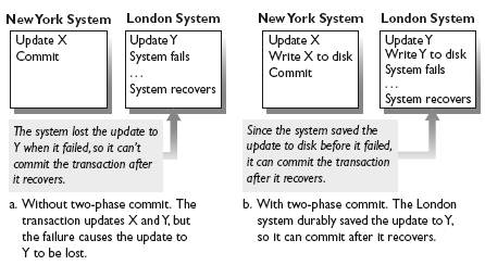 FIGURE 1.7 How Two-Phase Commit Ensures Atomicity. With two-phase commit, each system durably stores its updates before the transaction commits, so it can commit the transaction when it recovers.
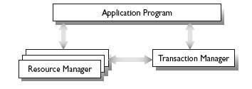 FIGURE 1.8 X/Open Transaction Model (XA). The transaction manager processes Start, Commit, and Abort. It talks to resource managers to run two-phase commit.
To understand two-phase commit, it helps to visualize the overall architecture in which the transaction manager operates. The standard model, shown in Figure 1.8 , was introduced by IBM's CICS and popularized by Oracle's Tuxedo and X/Open (now part of The Open Group, see Chapter 10). In this model, the transaction manager talks to applications, resource managers, and other transaction managers. The concept of "resource" includes databases, queues, files, messages, and other shared objects that can be accessed within a transaction. Each resource manager offers operations that must execute only if the transaction that called the operations commits.
FIGURE 1.8 X/Open Transaction Model (XA). The transaction manager processes Start, Commit, and Abort. It talks to resource managers to run two-phase commit.
To understand two-phase commit, it helps to visualize the overall architecture in which the transaction manager operates. The standard model, shown in Figure 1.8 , was introduced by IBM's CICS and popularized by Oracle's Tuxedo and X/Open (now part of The Open Group, see Chapter 10). In this model, the transaction manager talks to applications, resource managers, and other transaction managers. The concept of "resource" includes databases, queues, files, messages, and other shared objects that can be accessed within a transaction. Each resource manager offers operations that must execute only if the transaction that called the operations commits.
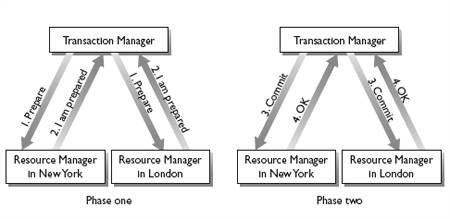 FIGURE 1.9 The Two-Phase Commit Protocol. In Phase One, every resource manager durably saves the transaction's updates before replying " I am Prepared. " Thus, all resource managers have durably stored the transaction's updates before any of them commits in phase two.
Two -phase commit avoids the problem in Figure 1.7(a) because all resource managers have a durable copy of the transaction's updates before any of them commit. Therefore, even if a system fails during the commitment activity, as the London system did in the figure, it can commit the transaction after it recovers. However, to make this all work, the protocol must handle every possible failure and recovery scenario. For example, in Figure 1.7(b) , it must tell the London system to commit the transaction. The details of how two-phase commit handles all these scenarios is described in Chapter 8.
Two -phase commit is required whenever a transaction accesses two or more resource managers. Thus, one key question that designers of TP applications must answer is whether or not to distribute their transaction programs among multiple resources. Using two-phase commit adds overhead (due to two-phase commit messages), but the option to distribute can provide better scalability (adding more systems to increase capacity) and availability (since one system can fail while others remain operational).
FIGURE 1.9 The Two-Phase Commit Protocol. In Phase One, every resource manager durably saves the transaction's updates before replying " I am Prepared. " Thus, all resource managers have durably stored the transaction's updates before any of them commits in phase two.
Two -phase commit avoids the problem in Figure 1.7(a) because all resource managers have a durable copy of the transaction's updates before any of them commit. Therefore, even if a system fails during the commitment activity, as the London system did in the figure, it can commit the transaction after it recovers. However, to make this all work, the protocol must handle every possible failure and recovery scenario. For example, in Figure 1.7(b) , it must tell the London system to commit the transaction. The details of how two-phase commit handles all these scenarios is described in Chapter 8.
Two -phase commit is required whenever a transaction accesses two or more resource managers. Thus, one key question that designers of TP applications must answer is whether or not to distribute their transaction programs among multiple resources. Using two-phase commit adds overhead (due to two-phase commit messages), but the option to distribute can provide better scalability (adding more systems to increase capacity) and availability (since one system can fail while others remain operational).
No comments:
Post a Comment